Phasor
In physics and engineering, a phase vector, or phasor, is a representation of a sine wave whose amplitude (A) and angular frequency (ω) are time-invariant. It is a subset of a more general concept called analytic representation. Phasors decompose the behavior of a sinusoid into three independent factors that relay amplitude, frequency and phase information. This can be particularly useful because the frequency factor (which includes the time-dependence of the sine wave) is often common to all the components of a linear combination of sine waves. In these situations, phasors allow this common feature to be factored out, leaving just the time-independent amplitude and phase information (the latter simply defining the phase at t=0 as θ), which can be combined algebraically rather than trigonometrically. Similarly, linear differential equations can be reduced to algebraic ones. The term phasor therefore often refers to just those two factors. In older texts, a phasor is also referred to as a sinor.
Contents |
Definition
Euler's formula indicates that sine waves can be represented mathematically as the sum of two complex-valued functions:
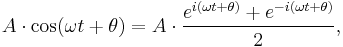
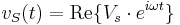
or as the real part of one of the functions:
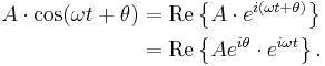
As indicated above, phasor can refer to either  or just the complex constant,
  . In the latter case, it is understood to be a shorthand notation, encoding the amplitude and phase of an underlying sinusoid.
An even more compact shorthand is angle notation: 
The sine wave can be understood as the projection onto the real axis of a rotating vector on the complex plane. The modulus of this vector is the amplitude of the oscillations, while its argument is the total phase  . The phase constant
  represents the angle that the complex vector forms with the real axis at t = 0.
Phasor arithmetic
Multiplication by a constant (scalar)
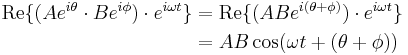
Multiplication of the phasor by a complex constant,  produces another phasor. That means its only effect is to change the amplitude and phase of the underlying sinusoid:
In electronics, would represent an impedance, which is independent of time. In particular it is not the shorthand notation for another phasor. Multiplying a phasor current by an impedance produces a phasor voltage. But the product of two phasors (or squaring a phasor) would represent the product of two sine waves, which is a non-linear operation that produces new frequency components. Phasor notation can only represent systems with one frequency, such as a linear system stimulated by a sinusoid.
Differentiation and integration
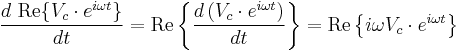
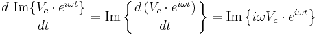
The time derivative or integral of a phasor produces another phasor.[2] For example:
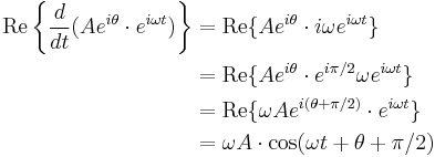
Therefore, in phasor representation, the time derivative of a sinusoid becomes just multiplication by the constant,  Similarly, integrating a phasor corresponds to multiplication by
  The time-dependent factor,
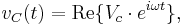
  , is unaffected. When we solve a linear differential equation with phasor arithmetic, we are merely factoring out of all terms of the equation, and reinserting it into the answer. For example, consider the following differential equation for the voltage across the capacitor in an RC circuit:
When the voltage source in this circuit is sinusoidal:
we may substitute:
where phasor  and phasor
  is the unknown quantity to be determined.
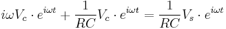
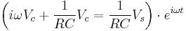
In the phasor shorthand notation, the differential equation reduces to[3]:
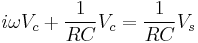
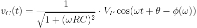
Solving for the phasor capacitor voltage gives:
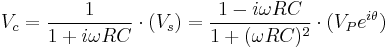
As we have seen, the factor multiplying  represents differences of the amplitude and phase of
  relative to
  and
and 
In polar coordinate form, it is:
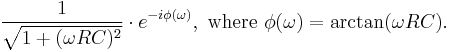
Therefore:
Addition
The sum of multiple phasors produces another phasor. That is because the sum of sine waves with the same frequency is also a sine wave with that frequency:
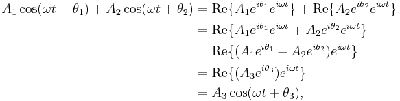
where:

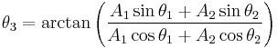
or, via the law of cosines on the complex plane (or the trigonometric identity for angle differences):

where  . A key point is that A3 and θ3 do not depend on ω or t, which is what makes phasor notation possible. The time and frequency dependence can be suppressed and re-inserted into the outcome as long as the only operations used in between are ones that produce another phasor. In angle notation, the operation shown above is written:

Another way to view addition is that two vectors with coordinates [A1 cos(ωt+θ1), A1 sin(ωt+θ1)] and [A2 cos(ωt+θ2), A2 sin(ωt+θ2)] are added vectorially to produce a resultant vector with coordinates [A3 cos(ωt+θ3), A3 sin(ωt+θ3)]. (see animation)
In physics, this sort of addition occurs when sine waves interfere with each other, constructively or destructively. The static vector concept provides useful insight into questions like this: "What phase difference would be required between three identical waves for perfect cancellation?" In this case, simply imagine taking three vectors of equal length and placing them head to tail such that the last head matches up with the first tail. Clearly, the shape which satisfies these conditions is an equilateral triangle, so the angle between each phasor to the next is 120° (2π/3 radians), or one third of a wavelength λ/3. So the phase difference between each wave must also be 120°, as is the case in three-phase power
In other words, what this shows is:

In the example of three waves, the phase difference between the first and the last wave was 240 degrees, while for two waves destructive interference happens at 180 degrees. In the limit of many waves, the phasors must form a circle for destructive interference, so that the first phasor is nearly parallel with the last. This means that for many sources, destructive interference happens when the first and last wave differ by 360 degrees, a full wavelength  . This is why in single slit diffraction, the minima occurs when light from the far edge travels a full wavelength further than the light from the near edge.
Phasor diagrams
Electrical engineers, electronics engineers, electronic engineering technicians and aircraft engineers all use phasor diagrams to visualize complex constants and variables (phasors). Like vectors, arrows drawn on graph paper or computer displays represent phasors. Cartesian and polar representations each have advantages.
Circuit laws
With phasors, the techniques for solving DC circuits can be applied to solve AC circuits. A list of the basic laws is given below.
- Ohm's law for resistors: a resistor has no time delays and therefore doesn't change the phase of a signal therefore V=IR remains valid.
- Ohm's law for resistors, inductors, and capacitors: V = IZ where Z is the complex impedance.
- In an AC circuit we have real power (P) which is a representation of the average power into the circuit and reactive power (Q) which indicates power flowing back and forward. We can also define the complex power S = P + jQ and the apparent power which is the magnitude of S. The power law for an AC circuit expressed in phasors is then S = VI* (where I* is the complex conjugate of I).
- Kirchhoff's circuit laws work with phasors in complex form
Given this we can apply the techniques of analysis of resistive circuits with phasors to analyze single frequency AC circuits containing resistors, capacitors, and inductors. Multiple frequency linear AC circuits and AC circuits with different waveforms can be analyzed to find voltages and currents by transforming all waveforms to sine wave components with magnitude and phase then analyzing each frequency separately, as allowed by the superposition theorem.
Power engineering
In analysis of three phase AC power systems, usually a set of phasors is defined as the three complex cube roots of unity, graphically represented as unit magnitudes at angles of 0, 120 and 240 degrees. By treating polyphase AC circuit quantities as phasors, balanced circuits can be simplified and unbalanced circuits can be treated as an algebraic combination of symmetrical circuits. This approach greatly simplifies the work required in electrical calculations of voltage drop, power flow, and short-circuit currents. In the context of power systems analysis, the phase angle is often given in degrees, and the magnitude in rms value rather than the peak amplitude of the sinusoid.
The technique of synchrophasors uses digital instruments to measure the phasors representing transmission system voltages at widespread points in a transmission network. Small changes in the phasors are sensitive indicators of power flow and system stability.
Footnotes
- ^
- i is the Imaginary unit (
 ).
). - In electrical engineering texts, the imaginary unit is often symbolized by j.
- The frequency of the wave, in Hz, is given by
 .
.
- i is the Imaginary unit (
- ^ This results from:
 which means that the complex exponential is the eigenfunction of the derivative operation.
 - ^ Proof:
-
(
Since this must hold for all
 , specifically:
  it follows that:
-
(
It is also readily seen that:
Substituting these into Eq.1 and Eq.2, multiplying Eq.2 by
 and adding both equations gives:
 -
References
- Douglas C. Giancoli (1989). Physics for Scientists and Engineers. Prentice Hall. ISBN 0-13-666322-2.